On the choice of output in model reference control

Abstract

This note discusses the choice of the output function when input-output linearizing.

\[ \newcommand{\tuple}[1]{ #1 } \newcommand{\d}{\mathrm d} \newcommand{\tp}[1]{{#1}^{\mathrm T}} \newcommand{\R}{\mathbb R} \]

Let’s investigate it using the example system, \[ m(x)\ddot x + r(x) \dot x + k(x) x = u, \] which in state-space form with state \(\tp{[x_1, x_2]} = \tp{[x, \dot x]}\) is \[ \begin{bmatrix} \dot x_1 \\ \dot x_2 \end{bmatrix} = \begin{bmatrix} \dot x \\ \frac 1{m(x)}[u - r(x)\dot x - k(x)x] \end{bmatrix}. \] If \(y = x_1 = x\), \[ \begin{aligned} \dot y &= \dot x_1 = x_2 \\ \ddot y &= \dot x_2 = \frac 1{m(x)}[u - r(x)\dot x - k(x)x] \\ \Leftrightarrow u &= m(x)\ddot y + r(x)\dot x + k(x)x. \end{aligned} \] If \(y = x_2 = \dot x\), \[ \begin{aligned} \dot y &= \dot x_2 = \frac 1{m(x)}[u - r(x)\dot x - k(x)x] \\ \Leftrightarrow u &= m(x)\dot y + r(x)\dot x + k(x)x. \end{aligned} \] So clearly, both choices of output will give the same input-output linearizing \(u\), but lead to systems with different relative degree. The smart choice is then to use the highest state derivative as output to reduce the number of differentiations.

Such a choice reduces JAX’s compilation times while leading to the exact same output law. Let’s look at an example using Dynax¹.

¹ The full source code of the example can be found here. Dynax is not yet released.

import time

import jax
import jax.numpy as jnp
import matplotlib.pyplot as plt
import numpy as np

from dynax import Flow, DynamicStateFeedbackSystem, ControlAffine
from dynax.linearize import relative_degree, input_output_linearize

We simulate a spring-mass damper with nonlinear drag, \[ m \ddot x + r \dot x + r_2 \dot x|\dot x| + k x = u. \] by bringing it into control-affine form \(\dot x = f(x) + g(x)u\).

class NonlinearDrag(ControlAffine):
  m: float
  r: float
  r2: float
  k: float
  n_states = 2
  n_inputs = 1
  n_outputs = 1

  def f(self, x, u=None, t=None):
    x1, x2 = x
    return jnp.array([
      x2,
      (-self.r * x2 - self.r2 * jnp.abs(x2) * x2 - self.k * x1) / self.m])

  def g(self, x, u=None, t=None):
    return jnp.array([0.0, 1.0 / self.m])

dyn = NonlinearDrag(m=1., r=1., r2=0.2, k=1.)
init_state = np.zeros(dyn.n_states)

The reference input is a sine at 0.1 Hz,

# design input signal
T = 100
sr = 100
t = np.arange(int(T*sr))/sr
r = 10*np.sin(2*np.pi*t*0.1)

and the reference dynamics is the nonlinear system linearized around \(x=0\).

ref_dyn = dyn.linearize()

fig, ax = plt.subplots(nrows=2)
ax[0].plot(r, label='$r$')
us = []

Let’s input-output linearize the system with either \(y=x_1=x\) or \(y=x_2=\dot x\):

for output in [0, 1]:
  # estimate relative degree
  x_test = np.random.normal(size=(1000, 2))
  reldeg = relative_degree(dyn, x_test, output=output)
  print("Relative degree:", reldeg)

  # construct input-output linearized model
  feedbacklaw = input_output_linearize(dyn, reldeg, ref=ref_dyn, output=output)
  feedbacksys = DynamicStateFeedbackSystem(dyn, ref_dyn, feedbacklaw)

  # combine model with ODE solver
  feedbackmodel = jax.jit(Flow(feedbacksys).__call__)
  init_xz = jnp.concatenate((init_state, init_state))

  # measure compile time
  start = time.time()
  xz, y_comp = feedbackmodel(init_xz, t, r)
  print(f"Compile+run: {time.time()-start}s")

  # measure jitted run time
  start = time.time()
  for i in range(5):
    xz, y_comp = feedbackmodel(init_xz, t, r)
  print(f"jitted run: {(time.time()-start)/5}s")

  # recompute u from states and input
  x, z = xz[:, :dyn.n_states], xz[:, dyn.n_states:]
  u = jax.vmap(feedbacklaw)(x, z, r)

  us.append(u)

  ax[0].plot(u, label=f'$u$ for $y=x[{output}]$')
  ax[1].plot(x[:, 0], label=f'$x$ for $y=x[{output}]$')
  ax[1].plot(z[:, 0], label=f'$z$ for $y=x[{output}]$')

for a in ax:
  a.legend()

plt.show()

which prints and plots:

Relative degree: 2
Compile+run: 2.477771520614624s
jitted run: 0.014502191543579101s
Relative degree: 1
Compile+run: 2.215977907180786s
jitted run: 0.014466238021850587s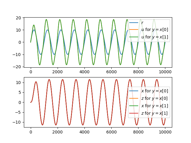

Note that two outputs are exactly the same:

np.all(us[0] == us[1])  # -> True

For larger models and time series, the compilation time can change quite considerably.